Simulation ( Continued )
In the schematic window of the hierarchical design, select " Analog Environment"
Click on Tools in the menu banner of the schematic entry window and choose Analog Environment.
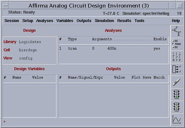
The Analog Environment main window will appears, as shown below. The main fields in this window which we are going to use are.
Note that the library, the cell and the view names are listed in the Design field, so that you can check that you are simulating the desired cell using the correct view.
Click on Setup in the menu banner and select Model Libraries.
Type in "$MODS/typ" and click on "add". You will observe that the library will be added. To save it click on "OK".
Also in the same Setup, click on Simulator/Directory/Host and select the simulator to be "spectreVerilog"
Click on Analyses in the menu banner and select Choose
Click on "tran" in the Analysis field.
There are many available analysis options you can choose. Each of these options provides a specific sub-region within the Choosing Analysis window. Since we want to obtain the delay information for the inverter, we choose the transient simulation type, so that the output can be traced in time domain. This may be a little bit different from what you see but it will differ much)
In the Transient Analysis region, type a value in the Stop Time field to determine how long the simulation will take place. The Stop Time is chosen 400n s (nanoseconds).
Note : Do not leave any space between the numeric value and the unit. Do not type "s" after the unit where "s" stands for "seconds".Do not forget to type a unit after the numeric value, otherwise, the stop time for the simulation will be something in seconds which means your simulation will last forever !
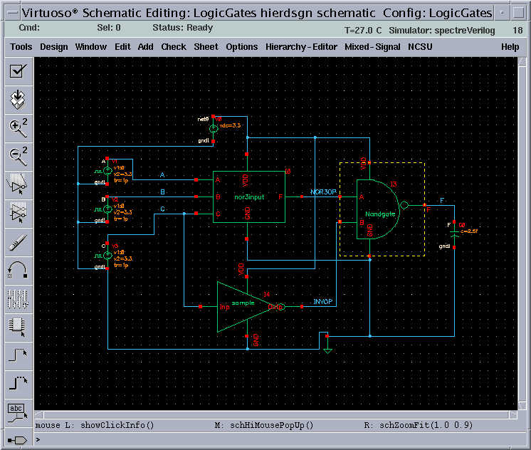
The schematic window will be as follows
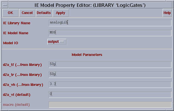
In the schematic window, click on the "Mixed - Signal" and select "Interface Nets" in the drop-Menu and select "library" from the drop menu. This will open the window shown below. Change the entries in the window as shown in the window below.
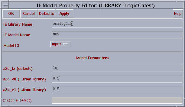
Select "input" in the "Model IO" and change the entries as shown in the window below.
Start the simulation by clicking Simulation and then selecting Netlist & Run.
The waveform window appears after the simulation is completed. It includes the waveforms of the selected nodes plotted between t=0 and the determined Stop Time which is 400 ns in our example.
After the simulation is run, we have to plot the output and the input. Now we will follow an other way to plot the input and output. Select "Results" in the "Affirma Analog Environment" window, select "Direct Plot" and select "Transient signal". We have to select the signals to be plotted from the schematic by clicking on corresponding wires and hit "Esc" on the keyboard. This will give the output from the wave form window.
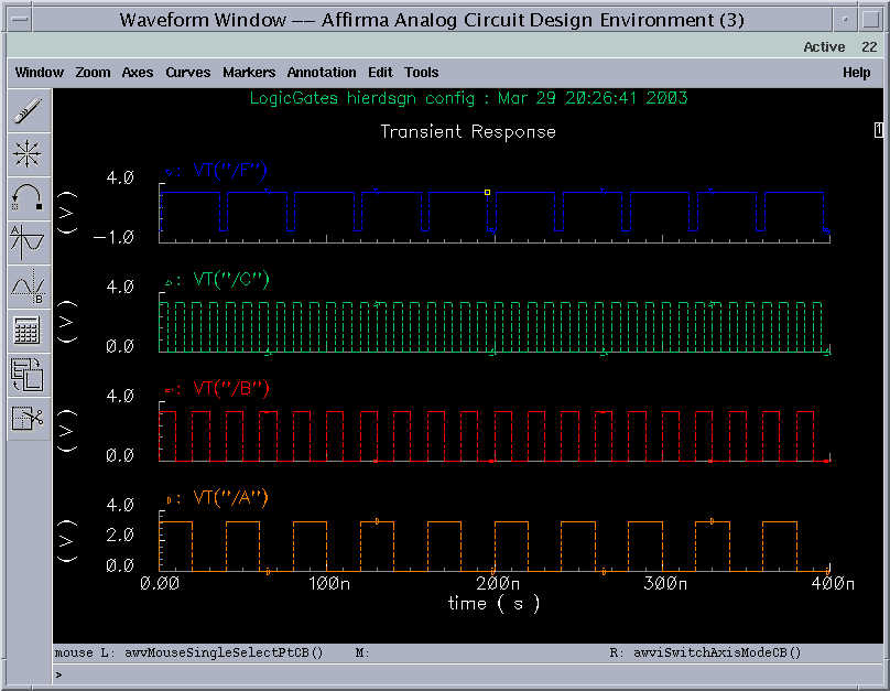
The results wave is shown above.
We can interchange the views of the three symbolic views in the hierarchy editor and rerun the simulation